Perform efficient Latent Semantic Index using Python
First of all, Latent Semantic Index(LSI) and Latent Semantic Analysis(LSA) are interchangeable terms. In E-discovery world, we often use LSI but in other fields, researchers often use LSA.
Latent semantic analysis is widely used in information retrieval to search for similar documents. In E-discovery doc review, finding similar documents can drastically decrease the number of documents case team have to review so it is a powerful and essential tool in today's E-discovery industry. LSI is the thing behind Relativity conceptual analytics.
Each document can have several topics and several words together can be used to express a topic. In another word, each document consists of a mixture of topics, and each topic consists of a collection of words. A word can appear several topics but the mixtures are different, i.e. bank appears in both "financial, money, bank" and "fishing, river, bank" topics, but the meaning of it is different. Please note the topics here are inferred and not observable, and that is why we use "latent" to describe them.
LSI is used to find the documents-topics and words-topics relationships. When we have the model formed, we can then find similar words that are used in any topic (keyword expansion), and similar documents that contain the similar topic mixtures (document classification). There are also other topic modeling techniques like pLSA, LDA and etc which i will write about in the future. For LSI, the pros and cons are for your reference.

Latent semantic analysis is widely used in information retrieval to search for similar documents. In E-discovery doc review, finding similar documents can drastically decrease the number of documents case team have to review so it is a powerful and essential tool in today's E-discovery industry. LSI is the thing behind Relativity conceptual analytics.
What is LSI and the intuition
The main idea of LSI can be generalized in one simple sentence: Words with similar meaning will occur in similar documents.Each document can have several topics and several words together can be used to express a topic. In another word, each document consists of a mixture of topics, and each topic consists of a collection of words. A word can appear several topics but the mixtures are different, i.e. bank appears in both "financial, money, bank" and "fishing, river, bank" topics, but the meaning of it is different. Please note the topics here are inferred and not observable, and that is why we use "latent" to describe them.
LSI is used to find the documents-topics and words-topics relationships. When we have the model formed, we can then find similar words that are used in any topic (keyword expansion), and similar documents that contain the similar topic mixtures (document classification). There are also other topic modeling techniques like pLSA, LDA and etc which i will write about in the future. For LSI, the pros and cons are for your reference.
The LSI overview
To implement LSA, we need to use bag of words (BOW) model.
- It is simply just generating a vocabulary for all the documents in corpus, and then generate a document-term matrix. Document-term matrix can be built in 1) simply binary way: if a term exists in the document, it's 1, otherwise, it's 0. 2) term count: the number of how many times a certain term shows in a particular document. 3) TF-IDF.
- After we have the matrix, we apply Singular Value Decomposition. SVD is an amazing algorithm which plays a very important role in IR and text classification. I will write about how to interpret SVD result of document-term matrix in the future because it is too much to talk about and beyond the scope of this tutorial.
- The last step is to determine the most optimal number of dimensions (number of topics) for the data set and reduce the SVD result to. This step is crucial because it not only removes the noisy topics but also forms topics from words via linear transformation. This step is called lower rank approximation.
LSI process
Most of LSI tutorials used several sentences as example to demonstrate. Surely it works for the purpose of demonstration but it does not provide audiences any insight of LSI performed on real world data. Thus, I chose to run on Enron emails. For this demonstration, i used a very standard machine (see below).
The total document count is ~220k. The Python packages I used to perform LSI are Pandas, NLTK, Matplotlib, and of course Sklearn. Since this tutorial is not a Python 101, i am not going to elaborate on each python snippets but just let you know what each step is for.
For pre-processing, i made all words to lower case, applied stemming so words so that words like applying, apply, applied are all reduced to its root: appli, and i also removed common English noise words. For documents, i excluded anything that has text size less than 5000 bytes, because documents with small text content usually bring nothing but noisy topics. In contrast to Relativity LSI which requires repeated contents to be removed from index, we do not need to do here because we will use TF-IDF model which will penalize words that appear too frequent. As matter of fact, TF-IDF is often the better choice than binary or count models.
Above is the code for pre-processing. After that, we can create a pandas dataframe to hold processed and tokenized content for each document, and feed into Sklearn tf-idf vectorizer. What Sklearn vectorizer gives us is a scaled document-word matrix, and it is ready to be fed into SVD.
Above is the code to perform the crucial SVD on our data. the console output and the plot are shown below. Please note i chose to reduce the dimension to 1750 from original 324,046. I will be explaining the reason why i chose this number which can be learned from the plot below.


There is a lot information above in the plot. Let me walk you through this:
So now, we can determine how to pick the number of dimensions. The logic is simply, if we have a lot of documents, say millions, we would keep the dimensions as small as possible, but try to keep sum of variance as big as possible. If we have not too many documents like in our case (only 22205), we could keep somewhere between 1500 and 2000. For this demo, i will pick 1750 which gives us 71.2% variance sum.

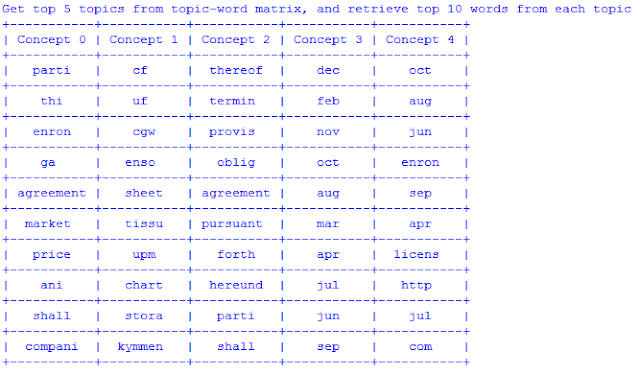
Keep in mind, concepts aka topics are more granular than the clusters we defined. One cluster can have a mixture of many topics. We can see both our model successfully grouped all months together. Words like "agreement", "party", "price" and "market" seem to be very related to one another. We also see several noise words we should remove like "enron", "www", "http", "shall" and etc. You will never notice them only until you run your model. We could add something in our pre-processing to remove them so it will generate a more accurate model. Remember, in real life, data scientist often runs with many iterations until it reaches an optimal model.
Above is the code to perform the crucial SVD on our data. the console output and the plot are shown below. Please note i chose to reduce the dimension to 1750 from original 324,046. I will be explaining the reason why i chose this number which can be learned from the plot below.

There is a lot information above in the plot. Let me walk you through this:
- The original document-word matrix contains 22205 documents, and 324046 words. Remember the beginning data set size is ~220k documents? The reason why it dropped nearly 90% of the documents is because we applied filter to include only documents that have text size over 5000 bytes. I could set the threshold lower, and I set it at 5000 mainly for two reasons: 1) to get more documents with decent amount of text, 2) to weed out as many as small documents so my demonstration could be run on a 16G memory machine ( : However, in real world, a good data scientist should spend most of his time in preparing data to determine a good threshold.
- To plot the graph, I initially set the dimension to 2500 (latent topics), so i can get a sense of variance recovery.
- The total sum of variance of 2500 latent topics give us 77.77% of original 324046 words variance. The intuition here could be interpreted as the 2500 latent topics still carry 77.77% information of original words. It is actually not bad.
- From the graph, we can see after ~600 dimensions, the plot is getting flat as increasing another 500 dimensions will only increase less than 10% of variance.
So now, we can determine how to pick the number of dimensions. The logic is simply, if we have a lot of documents, say millions, we would keep the dimensions as small as possible, but try to keep sum of variance as big as possible. If we have not too many documents like in our case (only 22205), we could keep somewhere between 1500 and 2000. For this demo, i will pick 1750 which gives us 71.2% variance sum.
Applications
After we performed truncated SVD, it gives us two things we can use: 1) (k dimension, n words) matrix, 2) (m documents, k dimension) matrix. From 1, we can calculate similarity between words based on their cosine similarity, or we can see list of tops words in each k topics. From 2, we can use same way to calculate document similarity, and see top documents for each k topics. Further more, you can apply another estimator on top of the result to get another layer "condensation" because the original latent topics are still very "granular". Since we do not have any labelled data in this set, so we can not perform any cross validation or nested cross validation to improve our model, nor could we perform any classification, I will stick with unsupervised learning algorithm to show you some aspects of the data. Below, I will demonstrate two things: 1) find top 10 words for first 5 concepts, 2) apply K-means to cluster the (m documents, k dimension) matrix into a more abstracted groups and find out top words in each cluster.
The result for 1) is shown below:
The result for 2) is shown below:
The result for 1) is shown below:

The result for 2) is shown below:


Comments
Post a Comment